使用 DuckDB 和 scikit-learn 进行机器学习原型开发
TL;DR: 在本文中,我们使用 DuckDB 进行数据处理,并使用 scikit-learn 进行模型构建,从而原型化一个机器学习工作流。
介绍
机器学习原型开发通常涉及数据集、预处理步骤和性能限制之间的平衡,这使得整个过程既复杂又耗时。scikit-learn 是 Python 最受欢迎和强大的机器学习库之一,提供了大量用于构建和评估模型的实用工具。在本文中,我们将通过在帕尔默群岛的企鹅观测数据上实现一个企鹅物种预测模型,探讨 DuckDB 如何在模型开发生命周期中补充 scikit-learn。
以下实现是在 marimo Python notebook 中执行的,该 notebook 可在我们的 示例仓库 的 GitHub 上获取。
数据准备
我们首先加载 Palmer Penguins 数据集,并使用 DuckDB 的 COLUMNS(*) 表达式 过滤掉任何包含 NA 或 NULL 的记录。
duckdb_conn.read_csv(
    "http://blobs.duckdb.org/data/penguins.csv"
).filter(
    "columns(*)::text != 'NA'"
).filter(
    "columns(*) is not null"
).select(
    "*, row_number() over () as observation_id"
).to_table(
    "penguins_data"
)
即使 NA 值已从数据集中移除,DuckDB 在 read_csv 时仍将列类型推断为 VARCHAR。因此,我们使用 ALTER TABLE 语句将列类型修改为数值类型 DECIMAL(5, 2)。
duckdb_conn.sql(
    "alter table penguins_data alter bill_length_mm set data type decimal(5, 2)"
)
提示:也可以在导入时 定义模式。
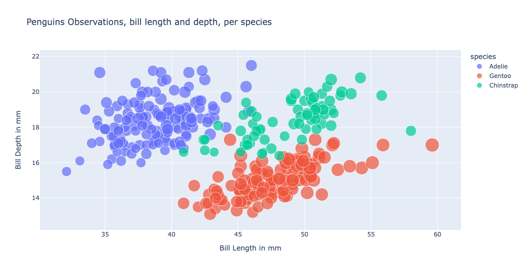
我们现在可以绘制数据并检查特定物种的聚类。例如,使用 散点图,我们可以在喙深度和喙长度的组合处识别出聚类。
我们还观察到数据集中有一些描述性列,例如 species 和 island。在机器学习工作流中,一个常见的预处理步骤是将这些值转换为数值,并为它们分配一个唯一标识符;这个过程称为 标签编码。虽然 scikit-learn 提供了 LabelEncoder 工具,但这个过程与我们在数据仓库中处理 参考表 的方式非常相似。因此,我们定义了一个函数,该函数将为每个列(特征)创建一个参考表,利用 DuckDB Python 关系型 API。
def process_reference_data(duckdb_conn):
    for feature in ["species", "island"]:
        duckdb_conn.sql(f"drop table if exists {feature}_ref")
        (
            duckdb_conn.table("penguins_data")
            .select(feature)
            .unique(feature)
            .row_number(
                window_spec=f"over (order by {feature})",
                projected_columns=feature
            )
            .select(f"{feature}, #2 - 1 as {feature}_id")
            .to_table(f"{feature}_ref")
        )
        duckdb_conn.table(f"{feature}_ref").show()
执行上述函数后,将创建两个表,其中包含类别的不同值和唯一标识符,例如 species_ref。
┌───────────┬────────────┐
│  species  │ species_id │
│  varchar  │   int64    │
├───────────┼────────────┤
│ Adelie    │          0 │
│ Chinstrap │          1 │
│ Gentoo    │          2 │
└───────────┴────────────┘
数据准备的最后一步是定义一个选择查询变量,该变量从初始数据集和参考表中选择数据。
selection_query = (
    conn.table("penguins_data")
    .join(conn.table("island_ref"), condition="island")
    .join(conn.table("species_ref"), condition="species")
)
selection_query是惰性求值的,因此在定义时不会检索数据。
模型训练
我们的目标是根据企鹅的特征(如喙长和喙深、鳍状肢长度、体重和岛屿)来预测其物种。这样的模型被称为分类模型,因为它预测输入数据所属的类别。scikit-learn 提供了 多种分类模型。对于我们的数据集,我们选择实现一个基于决策树的 随机森林分类器。
我们首先使用 scikit-learn 中的 train_test_split 工具 将数据分割成训练集和测试集。
def train_split_data(selection_query):
    X_df = selection_query.select("""
        bill_length_mm,
        bill_depth_mm,
        flipper_length_mm,
        body_mass_g,
        island_id,
        observation_id,
        species_id
    """).order("observation_id").df()
    y_df = [
        x[0]
        for x in selection_query.order("observation_id").select("species_id").fetchall()
    ]

    num_test = 0.30
    return train_test_split(X_df, y_df, test_size=num_test)

X_train, X_test, y_train, y_test = train_split_data(selection_query)
数据分割是机器学习工作流中的一个常见步骤,它返回以下内容:
X_train,包含我们希望基于其分配物种类别的输入数据;y_train,包含X_train中每个记录的物种;X_test,包含我们将用于测试模型的输入数据;y_test,包含X_test中每个记录的物种。
然后我们定义 RandomForestClassifier,并用 X_train 和 y_train 数据对其进行拟合。我们将模型保存在 pickle 文件中,以便无需重新训练即可使用该模型。
model = RandomForestClassifier(n_estimators=1, max_depth=2, random_state=5)

model.fit(X_train.drop(["observation_id", "species_id"], axis=1).values, y_train)

pickle.dump(model, open("./model/penguin_model.sav", "wb"))
我们现在可以检查模型的准确率分数。
model.score(
    X_test.drop(["observation_id", "species_id"], axis=1).values, y_test
)
0.98
由于我们的模型规模较小,我们使用
pickle。其他持久化方法在scikit-learn文档页面 中有详细说明。
使用 DuckDB 进行推理
推理是使用模型对(新)数据进行预测的过程。
model = pickle.load(open("./model/penguin_model.sav", "rb"))

model.predict(...)
使用 DuckDB 时,有三种方法可以从数据中检索预测类别。我们可以使用 Pandas,或者使用 DuckDB Python UDF(带或不带批处理)。接下来,我们将介绍这些方法。
使用 Pandas
检索预测最常用的方法是将预测加载到 Pandas 数据帧的新列中。
predicted_df = selection_query.select("""
    bill_length_mm,
    bill_depth_mm,
    flipper_length_mm,
    body_mass_g,
    island_id,
    observation_id,
    species_id
""").df()

predicted_df["predicted_species_id"] = model.predict(
    predicted_df.drop(["observation_id", "species_id"], axis=1).values
)
使用 DuckDB,数据帧可以通过 SQL 查询。
(
    duckdb_conn.table("predicted_df")
    .select("observation_id", "species_id", "predicted_species_id")
    .filter("species_id != predicted_species_id")
)
结果如下:
┌────────────────┬────────────┬──────────────────────┐
│ observation_id │ species_id │ predicted_species_id │
│     int64      │   int64    │        int64         │
├────────────────┼────────────┼──────────────────────┤
│             13 │          1 │                    2 │
│             15 │          1 │                    2 │
│             39 │          1 │                    2 │
│             44 │          1 │                    2 │
│             68 │          1 │                    2 │
│             70 │          1 │                    2 │
│             76 │          1 │                    2 │
│             90 │          1 │                    2 │
│             94 │          1 │                    2 │
│            104 │          1 │                    2 │
│            106 │          1 │                    2 │
│            110 │          1 │                    2 │
│            124 │          1 │                    2 │
│            126 │          1 │                    2 │
│            243 │          3 │                    2 │
│            296 │          2 │                    1 │
├────────────────┴────────────┴──────────────────────┤
│ 16 rows                                  3 columns │
└────────────────────────────────────────────────────┘
警告:如果存在与数据帧同名的表,则可以使用
register为数据帧指定另一个表名,例如duckdb_conn.register("table_name", predicted_df)。
DuckDB Python UDF,逐行处理
DuckDB 提供了从 Python 函数注册 用户定义函数(UDF) 的可能性。由于 UDF 是逐行执行的,我们的预测函数将为每一行返回预测的物种 ID。
def get_prediction_per_row(
    bill_length_mm: Decimal,
    bill_depth_mm: Decimal,
    flipper_length_mm: int,
    body_mass_g: int,
    island_id: int
) -> int:
    model = pickle.load(open("./model/penguin_model.sav", "rb"))
    return int(
        model.predict(
            [
                [
                    bill_length_mm,
                    bill_depth_mm,
                    flipper_length_mm,
                    body_mass_g,
                    island_id,
                ]
            ]
        )[0]
    )
在上述 Python 函数中,我们提供所需的特征作为模型的输入,并返回预测值(一个 integer)。有了这些信息,我们创建 DuckDB 函数。
duckdb_conn.create_function(
    "predict_species_per_row", get_prediction_per_row, return_type=int
)
我们现在可以在 SQL SELECT 子句中使用 UDF。
selection_query.select("""
    observation_id,
    species_id,
    predict_species_per_row(
        bill_length_mm,
        bill_depth_mm,
        flipper_length_mm,
        body_mass_g,
        island_id
    ) as predicted_species_id
""").filter("species_id != predicted_species_id")
这会返回与上述相同的结果。
DuckDB Python UDF,批处理样式
虽然逐行预测在获取少量行的预测时很有用,但在处理更多数据时性能会较差。因此,通过将数据聚合到数组中(保留顺序),我们可以模拟预测的大量检索(或批处理样式)。
我们首先创建一个 Python 函数,用于获取 JSON 对象的预测结果,该 JSON 对象包含作为模型输入所需的特征的列式表示。
def get_prediction_per_batch(input_data: dict[str, list[Decimal | int ]]) -> np.ndarray:
    """
    input_data example:
        {
            "bill_length_mm": [40.5],
            "bill_depth_mm": [41.5],
            "flipper_length_mm: [250],
            "body_mass_g": [3000],
            "island_id": [1]
        }
    """
    model = pickle.load(open("./model/penguin_model.sav", "rb"))

    input_data_parsed = orjson.loads(input_data)

    input_data_converted_to_numpy = np.stack(tuple(input_data_parsed.values()), axis=1)

    return model.predict(input_data_converted_to_numpy)


duckdb_conn.create_function(
    "predict_species_per_batch",
    get_prediction_per_batch,
    return_type=duckdb.typing.DuckDBPyType(list[int]),
)
尽管 DuckDB 具有
MAP和STRUCT数据类型,它们可以自动转换为字典,但与json_object相比(包括orjson反序列化时间),它们的执行时间更慢。
使用 json_object,我们提取特征的列式表示,格式为 'feature_name': array[feature]。
json_object(
    'bill_length_mm', array_agg(bill_length_mm),
    'bill_depth_mm', array_agg(bill_depth_mm),
    'flipper_length_mm', array_agg(flipper_length_mm),
    'body_mass_g', array_agg(body_mass_g),
    'island_id', array_agg(island_id)
) as input_data,
然后我们将预测结果与其他感兴趣的列打包到一个 STRUCT 中。
struct_pack(
    observation_id := array_agg(observation_id),
    species_id := array_agg(species_id),
    predicted_species_id := predict_species_per_batch(input_data)
) as output_data
最后,我们 unnest 结果,以便将列表展平为表。
.select("""
    unnest(output_data.observation_id) as observation_id,
    unnest(output_data.species_id) as species_id,
    unnest(output_data.predicted_species_id) as predicted_species_id
""")
上述查询被封装在一个名为 get_selection_query_for_batch 的 Python 函数中,我们可以用它来链式查询,例如,用于批量检索不正确的预测结果。
get_selection_query_for_batch(selection_query).filter("species_id != predicted_species_id")
批处理方法可以通过使用 LIMIT 和 OFFSET 循环遍历数据来实现。
for i in range(4):
    (
        get_selection_query_for_batch(
            selection_query
            .order("observation_id")
            .limit(100, offset=100*i)
            .select("*")
        )
        .filter("species_id != predicted_species_id")
    ).show()
LIMIT和OFFSET是最后执行的,因此它们应该在预测选择之前应用。
性能考量
为了获取大规模数据集的性能数据,我们生成了一个包含大约 5900 万条记录的虚拟数据集。在 16 GB MacBook Pro 上,对 10% 的 样本 进行批处理耗时在 3 到 4 秒之间,而 Pandas 实现则在 1 秒内完成。这是因为 Python UDF 包含多个转换步骤,影响了性能:
- 将输入数据解析为 JSON;
- 将 JSON 转换为 numpy 数组;
- 将数组展平为行。
我们仍然选择展示 Python UDF,因为它们在 Python 环境中工作时是一个强大的工具,而且在处理小数据时,性能差异可以忽略不计。
结论
在本文中,我们展示了 DuckDB 如何在机器学习开发生命周期中补充 scikit-learn,重点关注数据准备和推理阶段。虚拟数据上的推理结果不佳;这是模型的原因还是虚拟数据的原因?我们将这个问题留给读者,作为探索 DuckDB 如何用于模型评估和模型优化阶段的一种方式。

